Logits and LPMs

During a replication assignment for my statistics class this semester, I fit logit and linear probability models (LPMs) to two different dichotomous dependent variables (from this paper). The DVs were from the same dataset, and the analyzed samples were identical. Yet, the logit models consistently fit one DV better (both single and multilevel), and the LPMs fit the other DV better. The only real difference I saw between them was the proportion of 'successes' in each DV. That is, the proportion of 1s in DV. One DV had about 5% successes, the other about 23%. I decided to waste half a day test the relative fits of models on different proportions of successes.

So, I wrote a simulation that does a few things:

1. Generates three random variables with 10000 cases; one is normally distributed, two are binomial¹.
2. Generates a vector of probabilities, z, as a random function of those three variables (true $\beta$s are any integer between -2 and 2)
3. Converts z to log odds, and generates a DV, y, using those odds.
4. Then, it runs both an LPM and a logit using each of these variable sets
5. Rinse and repeat, 1000 times.

The code is below (and on Github). What you get on the back end is a list containing the logit objects, and a list containing the LPM objects. It's easy then to extract the BICs from each model pair and compare them. Below is a graph of the results. The x-axis is the proportion of a given sample that are 'successes'; the y-axis is the BIC of the LPM minus the BIC from the logit. Positive values of the y-axis indicate superior fit by the logit model, negative values indicate better fit by the LPM.

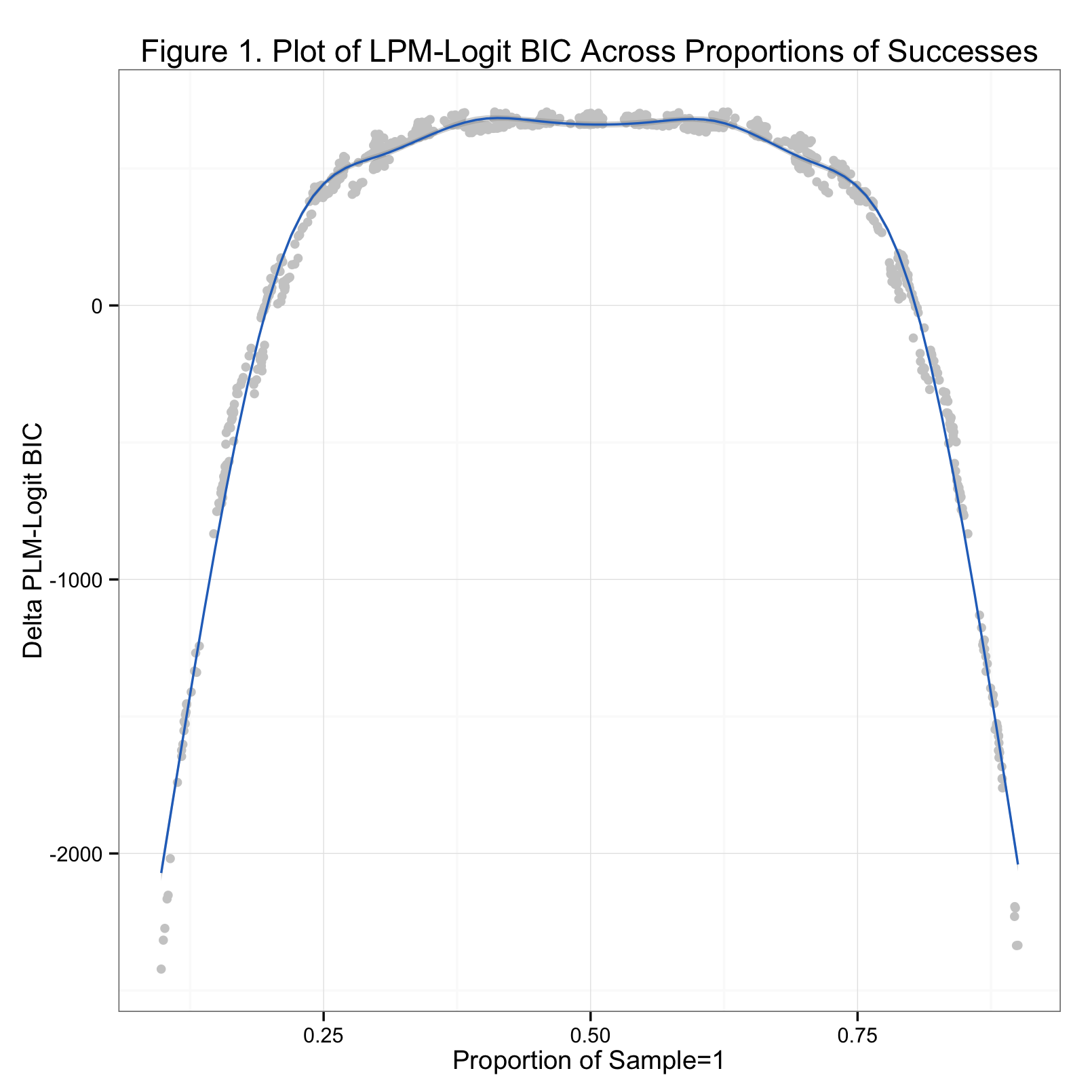
It's clear from the graph that neither model wins universally. As we might expect, the logit model fits the data better when the proportion of probabilities is between about 0.15 and 0.85. Astute observers will realize that these tails correspond to the flattening points on the logit curve. It appears that if proportion of successes in the sample falls within one of these tails, the logit has a worse and worse time fitting the data as the proportion approaches 0 or 1.

Based on a suggestion by a fan of LPMs here in the Triangle area, I also tested the models on a linearly-defined binomial outcome. The thought was that the function used to define probability affected the outcome - a logit should fit a logit-shaped probability better. So, I ran another simulation (code below) that defined probability linearly. The big reveal is that it doesn't affect the outcome:

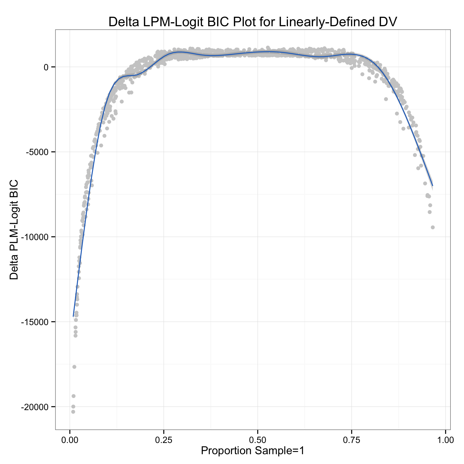
So, regardless of the "true" shape of latent probability, the logit fits the data better for most of the proportions of successes. Also interesting are the upper bounds of the curves, about 750 on the first plot, 1000 on the second - meaning the logit can't beat the LPM by more than this. A BIC of 750-1000 is still pretty big, no matter the context. The real peril comes when using logits on data with fewer than 15% or more than 85% positive cases. In these situations, the LPM fits better than the logit by ~2000 or even ~8000 'BIC points' (if I may).

The problem, though, is that sociologists (and probably social scientists more broadly) are generally interested in rare outcomes. We don't want to know the probability someone will stay in their home country, we want to know the probability that someone will migrate. Even "common" cases like incarceration and college graduation fall at or below the 15% threshold. This means sociologists in particular ought to be wary of using logits with abandon.

I should note that in my particular results, the difference in fit didn't produce different substantive results (read: differences in statistical significance) - robustly significant variables (p<0.01) were significant in all models. However, I would be particularly wary of logit coefficients with sig. values of p<0.05 from a logit model on DVs with proportions of successes less than 0.15. Happy summer.

Code

library("ggplot2")

# Inverse-Logit Probability Simulation
nreps = 1000
glms <- vector("list", length(nreps))
lms <- vector("list", length(nreps))
tots <- vector("list", length(nreps))
cs <- sample(-2:2, 1000, replace = T)
for (i in 1:nreps) {
    x <- rnorm(10000)
    x1 <- rbinom(10000, 1, sample(0.9))
    x2 <- rbinom(10000, 1, sample(0.6))
    z <- sample(cs, 1) * x + sample(cs, 1) * x1 + sample(cs, 1) * x2 + rnorm(10000)
    pr = 1/(1 + exp(-z))
    y = rbinom(10000, 1, pr)
    glms[[i]] <- glm(y ~ x + x1, family = binomial(link = "logit"))
    lms[[i]] <- lm(y ~ x + x1)
    tots[[i]] <- sum(y == 1)
}

# Construct Comparison Matrix for Plot
thecomp <- cbind(unlist(lapply(glms, function(x) BIC(x))), unlist(lapply(lms, 
    function(x) BIC(x))), unlist(lapply(tots, function(x) x/10000)))
thecomp <- as.matrix(thecomp)
thecomp <- cbind(thecomp, (thecomp[, 2] - thecomp[, 1]))
thecomp <- as.data.frame(thecomp)

# Linear Probability Simulation
nreps=1000
glms2<-vector('list', length(nreps))
lms2<-vector('list', length(nreps))
tots2<-vector('list', length(nreps))
cs<-sample(-2:2,1000,replace=T)
decider<-runif(1000,0,1)
printnums=seq(from=0, to=nreps, by=10)
for(i in 1:nreps){
  x<-rnorm(10000)
  x1<-rbinom(10000,1,sample(0.9))
  x2<-rbinom(10000,1,sample(0.6))
  z<-sample(cs,1)*x + sample(cs,1)*x1+ sample(cs,1)*x2 +rnorm(10000)
  y = ifelse((z>sample(decider,1)),1,0)
  glms2[[i]]<-glm(y~x+x1,family=binomial(link='logit'))
  lms2[[i]]<-lm(y~x+x1)
  tots2[[i]]<-sum(y==1)
  if(i %in% printnums) cat(i)
  else cat(".")
}


# Build Matrix for Plot, Simulation 2
thecomp2<-cbind(unlist(lapply(glms2,function(x) BIC(x))),unlist(lapply(lms2,function(x) BIC(x))),unlist(lapply(tots2, function(x) x/10000)))
thecomp2<-as.matrix(thecomp2)
thecomp2<-cbind(thecomp2, (thecomp2[,2]-thecomp2[,1]))
thecomp2<-as.data.frame(thecomp2)

# Simulation 1 Plot
p <- ggplot(thecomp)
p <- p + geom_point(aes(x = V3, y = V4), color = "#CCCCCC") + 
geom_smooth(aes(x = V3, y = V4), color = "#2671C4") + theme_bw() + xlab("Proportion of Sample=1") + ylab("Delta PLM-Logit BIC") + 
ggtitle("Figure 1. Plot of LPM-Logit BIC Across Proportions of Successes")

# Simulation 2 Plot
p.2<-ggplot(thecomp2)
p.2<-p.2+geom_point(aes(x=V3,y=V4),color="#CCCCCC")+
geom_smooth(aes(x=V3,y=V4),color="#2671C4")+theme_bw()+
xlab("Proportion Sample=1")+ylab("Delta PLM-Logit BIC")+
ggtitle("Delta LPM-Logit BIC Plot for Linearly-Defined DV")